In summary, this code provides a comprehensive guide on using a CNN to label audio data, from data loading and preprocessing to model training, evaluation, and prediction on new audio samples.
Let’s import all the required Python modules as the first step:
import os
import librosa
import numpy as np
import tensorflow as tf
from tensorflow.keras.layers import Input, Conv2D, MaxPooling2D, Flatten, Dense
from tensorflow.keras.models import Model
from tensorflow.keras.optimizers import Adam
from sklearn.model_selection import train_test_split
from tensorflow.keras.utils import to_categorical
from tensorflow.image import resize
from tensorflow.keras.models import load_model
Step 1: Load and preprocess data: Now, let’s load and pre-process the data for cats and dogs. The source of this dataset is https://www.kaggle.com/datasets/mmoreaux/audio-cats-and-dogs:
Define your folder structure
data_dir = ‘../cats_dogs/data/’
classes = [‘cat’, ‘dog’]
This code establishes the folder structure for a dataset containing the ‘cat’ and ‘dog’, categories, with the data located at the specified directory, ‘../cats_dogs/data/’. Next, let’s pre-process the data:
define the function for Load and preprocess audio data
def load_and_preprocess_data(data_dir, classes, target_shape=(128, 128)):
data = []
labels = []
for i, class_name in enumerate(classes):
class_dir = os.path.join(data_dir, class_name)
for filename in os.listdir(class_dir):
if filename.endswith(‘.wav’):
file_path = os.path.join(class_dir, filename)
audio_data, sample_rate = librosa.load(file_path, sr=None)
Perform preprocessing (e.g., convert to Mel spectrogram and resize)
mel_spectrogram = \
librosa.feature.melspectrogram( \
y=audio_data, sr=sample_rate)
mel_spectrogram = resize( \
np.expand_dims(mel_spectrogram, axis=-1), \
target_shape)
print(mel_spectrogram)
data.append(mel_spectrogram)
labels.append(i)
return np.array(data), np.array(labels)
This code defines a function named load_and_preprocess_data that loads and preprocesses audio data from a specified directory. It iterates through each class of audio, reads .wav files, and uses the Librosa library to convert the audio data into a mel spectrogram. We learned about the mel spectrogram in Chapter 10 in the Visualizing audio data with Matplotlib and Librosa – spectrogram visualization section.
The mel spectrogram is then resized to a target shape (128×128) before being appended to the data list, along with the corresponding class labels. The function returns the preprocessed data and labels as NumPy arrays.
Step 2: Split data into training and testing sets: This code segment divides the preprocessed audio data and corresponding labels into training and testing sets. It utilizes the load_and_preprocess_data function to load and preprocess the data. The labels are then converted into one-hot encoding using the to_categorical function. Finally, the data is split into training and testing sets with an 80–20 ratio using the train_test_split function, ensuring reproducibility with a specified random seed:
Split data into training and testing sets
data, labels = load_and_preprocess_data(data_dir, classes)
labels = to_categorical(labels, num_classes=len(classes)) Convert labels to one-hot encoding
X_train, X_test, y_train, y_test = train_test_split(data, \
labels, test_size=0.2, random_state=42)
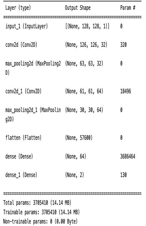
Step 3: Create a neural network model: This code defines a neural network model for audio classification. The model architecture includes convolutional layers with max pooling for feature extraction, followed by a flattening layer. Subsequently, there is a dense layer with ReLU activation for further feature processing. The final output layer utilizes softmax activation to produce class probabilities. The model is constructed using the Keras functional API, specifying the input and output layers, and is ready to be trained on the provided data:
Create a neural network model
input_shape = X_train[0].shape
input_layer = Input(shape=input_shape)
x = Conv2D(32, (3, 3), activation=’relu’)(input_layer)
x = MaxPooling2D((2, 2))(x)
x = Conv2D(64, (3, 3), activation=’relu’)(x)
x = MaxPooling2D((2, 2))(x)
x = Flatten()(x)
x = Dense(64, activation=’relu’)(x)
output_layer = Dense(len(classes), activation=’softmax’)(x)
model = Model(input_layer, output_layer)
Step 4: Compile the model: This code compiles the previously defined neural network model using the Adam optimizer, with a learning rate of 0.001, categorical cross-entropy as the loss function (suitable for multi-class classification), and accuracy as the evaluation metric. The model.summary() command provides a concise overview of the model’s architecture, including the number of parameters and the structure of each layer:
Compile the model
model.compile(optimizer=Adam(learning_rate=0.001), \
loss=’categorical_crossentropy’, metrics=[‘accuracy’])
model.summary()
Here is the output:

Figure 11.5 – Model summary